In this tutorial, I will show you how to extract several important metrics from a thermal map or image and how to derive landscape patterns and calculate different landscape diversity indices. We are going to use the quite new and experimental QGIS3 plugin ThermalMetrics.
IMPORTANT: Since this is still the experimental version of the plugin, it will undergo further testing. I will also add more functionality (such as more indices and more patch metrics) with the next versions soon. If you find a bug or encounter any other problem, please tell me about it. I am happy for every idea of how to improve the plugin and this workflow.
You will learn:
- how to install the free and open source QGIS3 plugin ThermalMetrics
- how to calculate a set of metrics to better understand the temperature distribution of your thermal maps and images
- how to derive patches and patterns from the temperatures in your map or image
- how to calculate the Shannon Diversity Index, the Simpson Diversity Index and many more indices, based on the derived patches
Let’s start with some background. You can skip this section if you are looking for fast results. I also might have simplified some of the rather complex relationships here to keep it short and understandable.
What are the most common metrics to describe land surface temperatures?
The choice of metrics highly depends on your question and what you find most interesting about the ecosystem or landscape, that was recorded in your thermal data. However, there is a set of indices that is almost always need as a statistical backbone for any analysis. You might want to start with the technical map or image details, such as the total number of pixels in the map and the total number of non-NaN pixels, i.e. pixels that actually represent temperature values and that are not just empty. The relation of empty and not empty pixels and the overall shape of the map in the x and y direction are also quite interesting. Moreover, geographic metrics such as the area covered by your map and covered by the data are important when comparing different maps. Simple statistical metrics such as minimum, maximum and mean temperature (in K and °C), the standard deviation and variance of temperature provide further insights into the represented temperatures.
However, statistics such as means and variance will always summarize the map as a whole. Distribution metrics are the key to look deeper into the actual distribution of temperatures. A histogram separates the data into a set of groups or bins that fall between margins. Skewness, Kurtosis and coefficients such as the Fisher-Pearson Coefficient of Skewness (FPCS) allow to assess how the data are distributed.
The study of microclimate and thermal heterogeneity based on land surface temperatures requires to derive patches from the thermal maps. Patches are smaller areas with a very similar behavior or thermal pattern. Imagine an agricultural landscape. You might have several fields with different crops: wheat, corn, potatoes and sugar beet. You might also have a small grove, a hedge and a farm road to access them all. All of these areas represent very different microclimates and they will look very different when represented by a thermal landscape temperature map. The grove might be colder than the farm road on a sunny day, because trees transpirate more water than the small herbs and grasses growing on the farm road. The hedge might have a much more diverse microstructure than the field of wheat. This can all be represented by patches. The calculation of thermal patches can help to further analyze these heterogenous landscapes. If you need to compare different landscapes, sites or plots, you will need to normalize your information in some way, to make it comparable with other maps. Here diversity indices come in handy. The most common diversity indices are the Shannon Diversity Index and the Simpson Diversity Index. Depending on what exactly you want to know about your maps, sites and plots, other very similar indices such as the Shannon Equitability Index, the Gini-Simpson Diversity Index and the Simpson Reciprocal Index might also be interesting.
This tutorial covers how to calculate all of these metrics and indices from your thermal images and maps. So, let’s get started.
How to calculate metrics and indices from thermal images?
To efficiently calculate thermal metrics and diversity indices, we first need to install the necessary software.
We are going to work with the free QGIS3 software. You can download it here. From my experience, I can recommend to use the “full OSGeo4W Network Installer”, because it installs many very useful dependencies too.
Any QGIS3 version should work, QGIS2 versions will NOT work. Follow the steps in the installation guide and open the QGIS3 canvas.
Install the experimental ThermalMetrics plugin
With QGIS3 installed, and opened, go to the tab Plugins and then to “Manage and Install Plugins…”:
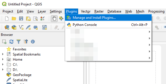
Click on “Manage and Install Plugins…” and open the plugin manager.
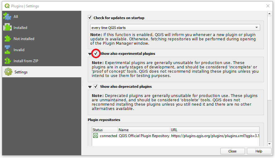
Since we are going to install an experimental plugin, first go to Settings and tick the check box “Show also experimental plugins”
Then click on “All”, and type “ThermalMetrics” into the search box. The ThermalMetrics plugin should then be ready to install.
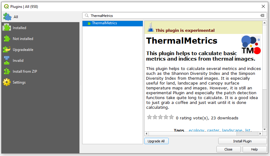
To install the ThermalMetrics plugin click on “Install Plugin”. The Plugin should then be installed and be ready to use. You can close the plugin manager now. In this tutorial we work with version 0.1 of the ThermalMetrics plugin, but later versions should work very similar.
Calculating thermal metrics and diversity indices with the ThermalMetrics plugin
To open the ThermalMetrics plugin, you can either select the tab Plugins and then navigate in the drop down menu to ThermalMetrics or you can quickly click on the ThermalMetrics icon among your installed plugins.
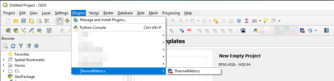
The ThermalMetrics GUI will now open.

How to fill the GUI:
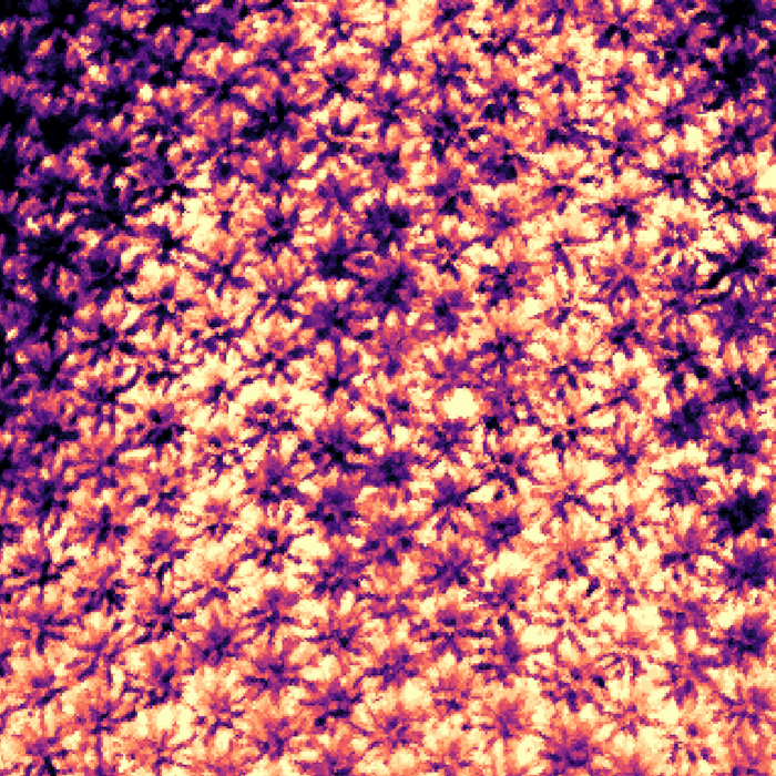
To run the ThermalMetrics plugin you’ll need an image or a map with land surface temperatures e.g. of a landscape with fields, hedges and farm roads. This image can be recorded by satellite, plane, drone or by a handheld thermal camera. You can either use your own georeferenced, single-band raster, where each pixel represents a temperature measurement either in Kelvin or degree Celsius, or you can download an example picture here.
(1) To load the thermal image, please use “Select input raster” to search and define your input image on your computer. If this step was successful, you should now see your map on the QGIS3 canvas.
(2) Define the path for the output file that contains the output information.
(3) If your thermal image contains empty values, you can define them in this step. This is an optional step. You don’t need to specify anything if there are no empty values in your image or if these empty values are either 0 or None.
(4) Many of the features such as the simple geographic metrics and the distribution section are already ticked by default.
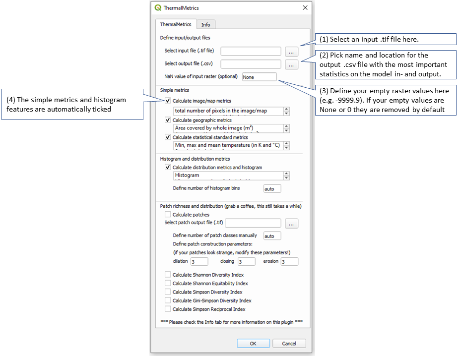
Now click OK and run the thermal metrics calculation. After a few seconds, a .csv file will be created that contains all the metrics.
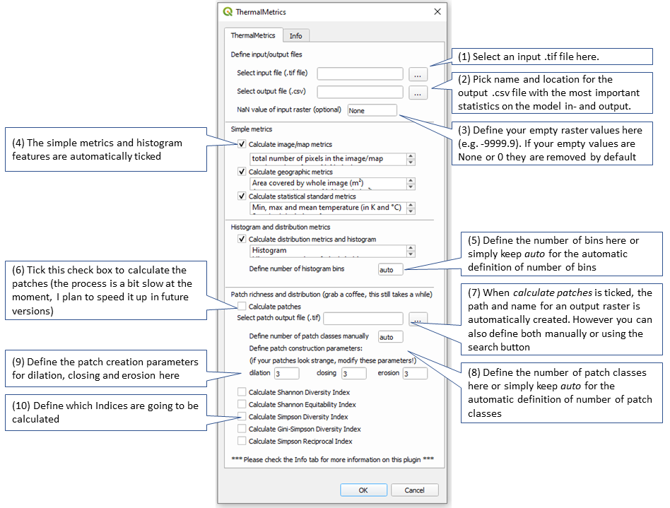
Calculating landscape patches and indices:
(5) For a first test run, the auto function to define the number of histogram bins worked fine. However, you can also define the number of bins manually. Just type in a bin number such as 10, 15 or 50.
(6) To calculate the landscape patches, tick the calculate patches check box. If it is checked, a path and an output file name are created automatically. You can also rename that file and redefine that path using the search button in (7) or by simply typing in the textbox.
(8) The number of patch classes (a patch class is a range between two margins from which a set of values is differentiated from other values) is defined automatically by default. However, you can also define these classes manually.
(9) The patch construction parameters can be defined manually using three text boxes, for dilation, closing and erosion. The patch construction parameters help to construct the individual patches. They are by default all set to 3, because that resulted to be a good compromise for my test rasters. Generally, pick higher numbers (try 8 or 20) if your patches are supposed to be bigger (e.g. if you want a wheat field to be one entire patch and the road and hedge next to it to also be single patches for themselves, especially when you are using high resolution images). If you are interested in selecting the single plants in your wheat field, then you should pick a lower value. 1 is the minimum though.
You can also choose three different values, e.g. dilation = 4, closing = 3, erosion = 15 if that works better for you. I plan to also provide an automated selection feature here in the future.
(10) Finally, you can define which indices you want to calculate based on the patches. The Indices are deactivated by default. The Shannon Diversity Index is a pretty common index in ecology, my implementation of this index and the similar indices the Shannon Equitability Index and the Shannon Equitability Index are based on this and this source. The Simpson Diversity Index is also frequently used in ecology, my implementation of this index and the similar indices, the Gini-Simpson Diversity Index and the Simpson Reciprocal Index are based on this and this source.
Now click OK and run the metrics and indices calculation. After a few seconds, a new layer will appear on top of the thermal image. This new raster layer is the result layer that contains the patches. Your raster is saved as a .tif file and the statistics are saved in a .csv file in the location that you specified in step (2) and (7). A second .csv file is created with the individual patch details and saved at the location specified in (2). I plan to add further parameters for the patches with future versions of this plugin.
Did you encounter problems? Or did you find a bug?
As I mentioned already, the plugin is currently still under development and there will be more features in the future. I am always happy to help and I am even happier to remove bugs from the software. Just write me.
How to cite the ThermalMetrics plugin?
If you are using this plugin for a scientific publication please carefully check if your results are realistic since we didn’t thoroughly check the plugin with a wide range of data yet and don’t forget to cite it accordingly using:
Ellsäßer, F. (2021) QGIS3 ThermalMetrics Plugin version 0.1 URL: https://plugins.qgis.org/plugins/thermalmetrics/
More Information
The ThermalMetrics plugin is the result of a few rainy evenings during the last year. I was just curious of how to calculate a set of indices and metrics from thermal images and I just kept developing it for myself. Since I realized that there was no simple tool that would do all these things out there, I decided to publish it as a QGIS3 plugin. I don’t claim that it is perfect yet and due to its simplicity, I cannot guarantee that it will work under all conditions. If you have any suggestions, ideas for improvement or further development, did you find a bug or do you want to contribute to the Ecosystem Respiration Tool project, please feel free to contact me.
You can find the Ecosystem Respiration Tool repository here.