There are a few tutorials around that help you calculate evapotranspiration from thermal images. This one is different because it is fully based on free and open source software, it is designed to be simple and focused on the actual task.

You will learn:

• how evapotranspiration is connected to canopy and land surface temperatures
• how to install the free open-source software required
• how to calculate evapotranspiration from thermal images
• how to improve your results

Let’s start with some background. You can skip this section if you are looking for fast results. I also might have simplified some of the rather complex relationships here to keep it short and understandable.

What is evapotranspiration and how is it connected to land and canopy temperatures?

Evapotranspiration is the sum of evaporation and transpiration of water from a surface to the atmosphere. With the evapotranspiration of water, both water and energy are transferred from the plant or soil to the atmosphere, cooling the surface – a process, which is called evaporative cooling. Therefore, surface temperatures can be a great indicator for evapotranspiration. Colder plant surface temperatures can therefore be an indicator for more evaporative cooling and hence more water being evapotranspirated from the surface to the air. Higher temperatures can be caused by a lower evapotranspiration and hence indicate a lack of water or just a dry surface.

How to calculate Evapotranspiration from thermal images?

Evapotranspiration models help to calculate actual evapotranspiration from thermal images. To apply such a model, we first need to install the necessary software.

We are going to work with the free QGIS3 software. You can download it here.  From my experience, I can recommend you to use the full OSGeo4W Network Installer, because it installs many very useful dependencies too.

Any QGIS3 version should work, QGIS2 versions will NOT work. Follow the steps in the installation guide and open the QGIS3 canvas.

Install the QWaterModel plugin

With QGIS3 installed, and opened, go to the tab Plugins and then to “Manage and Install Plugins…”:

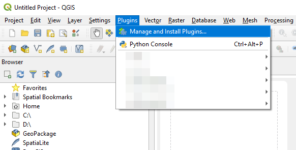
Click on “Manage and Install Plugins…” and open the plugin manager.

In the plugin manager click on “All”, then type “QWaterModel” into the search box. The QWaterModel Plugin should then be ready to install.

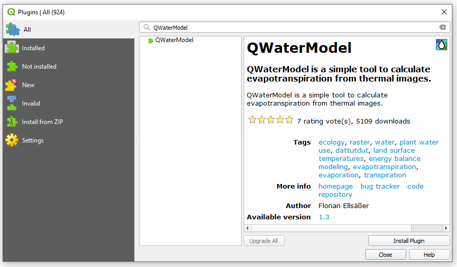
To install the QWaterModel plugin click on “Install Plugin”. The Plugin should then be installed and be ready to use. You can close the plugin manager now. In this tutorial we work with version 1.3 but later versions should work very similar.

Calculating Evapotranspiration with QWaterModel

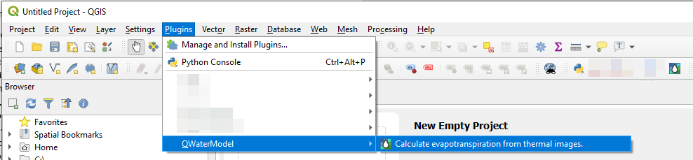
Open the QWaterModel plugin now to calculate Evapotranspiration from your thermal images. To open the plugin, you can either select the tab Plugins and then navigate in the drop down menu to QWaterModel or you can quickly click on the QWaterModel icon among your installed plugins.

The QWaterModel GUI will now open:

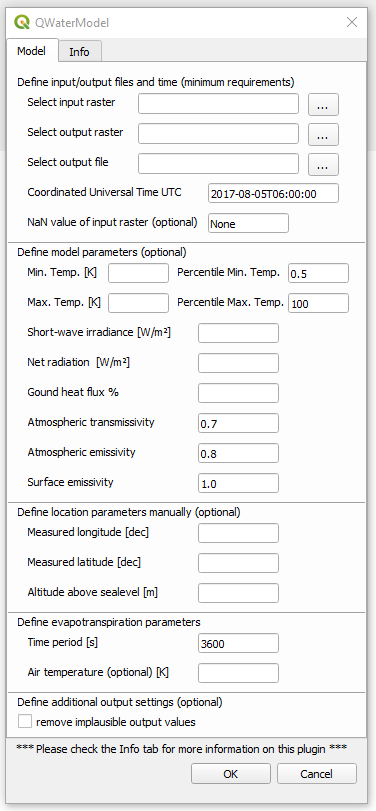
The minimal approach to calculate evapotranspiration:

For a first test run, we just need a thermal picture and the time (UTC) it was taken. You can either use your own georeferenced, single-band raster, where each pixel represents a temperature measurement either in Kelvin or degree Celsius, or you can download an example picture here.

(1) To load the thermal image, please use “Select input raster” to search and define your input image on your computer. If this step was successful, you should now see your map on the canvas.

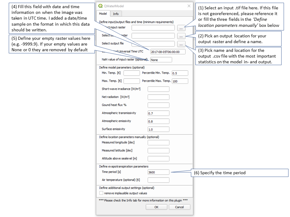
(2 and 3) Define the path for the output raster and the output file that contains the output information too.

(4) Then define the time the picture was taken in the UTC time format. The default is: year-month-dayThour:minute:second. This could look like this: 2021-05-01T11:00:00 for 11am coordinated universal time on 1^st of May in 2021.

(5) If your thermal image contains empty values, you can define them in this step. This is an optional step. You don’t need to specify anything if there are no empty values in your image or if these empty values are either 0 or None.

(6) A very important point is to specify the time period (in seconds) for which you want to calculate the evapotranspiration. The default is one hour (3600 seconds). From my experience, I can’t recommend to extend this time period for more than 3 hours, since your thermal map represents only a snapshot of a certain day. Evapotranspiration can change very fast. Covering many hours or even a full day of evapotranspiration, based on a single image, will most likely result in a very inaccurate estimate. It is better to use several images or maps per day if this is possible or to think about a very representative time of the day (e.g. 10 am) that might represent a good average evapotranspiration.

Now click OK and run the evapotranspiration model. After a few seconds, a new layer will appear on top of the thermal image. This new raster layer is the result layer. It contains six-bands with the model results:

Band 1: net radiation Rn [W/m²]

Band 2: latent heat flux LE [W/m²]

Band 3: sensible heat flux H [W/m²]

Band 4: ground heat flux G [W/m²]

Band 5: evaporative fraction EF [%/100]

Band 6: evapotranspiration ET [kg/time period]

Your raster is saved as a .tif file and the statistics are saved in a .csv file in the location that you specified in step (2 and 3).

How to interpret these results?

Now you have your first evapotranspiration estimate. But since it is based on only very little data input, there is lots of room for improvement. The model that generated these first results didn’t have enough data to account for clouds or actual air temperature. Therefore, these values have been estimated. However, your results might still be quite accurate now, if your thermal picture or map was recorded on a sunny day without clouds around noon. In the following step, you’ll see how you can improve your evapotranspiration estimates.

How to improve your results?

In this step, we will significantly improve the accuracy of your evapotranspiration estimates. The idea of this section is very simple: the more data you provide to QWaterModel, the closer your estimates are to the real world.

(7) Sometimes there are artifacts or unwanted objects in your image. These objects could be a very warm stone in the middle of a field or a shiny metal surface that reflects the space temperature and appears to be really cold. There are several options to exclude these. The most common is to use a mask layer and to just remove them from your thermal map. However, here you can remove them by manually adding minimum or maximum values or the respective thresholds with which they are generated automatically.

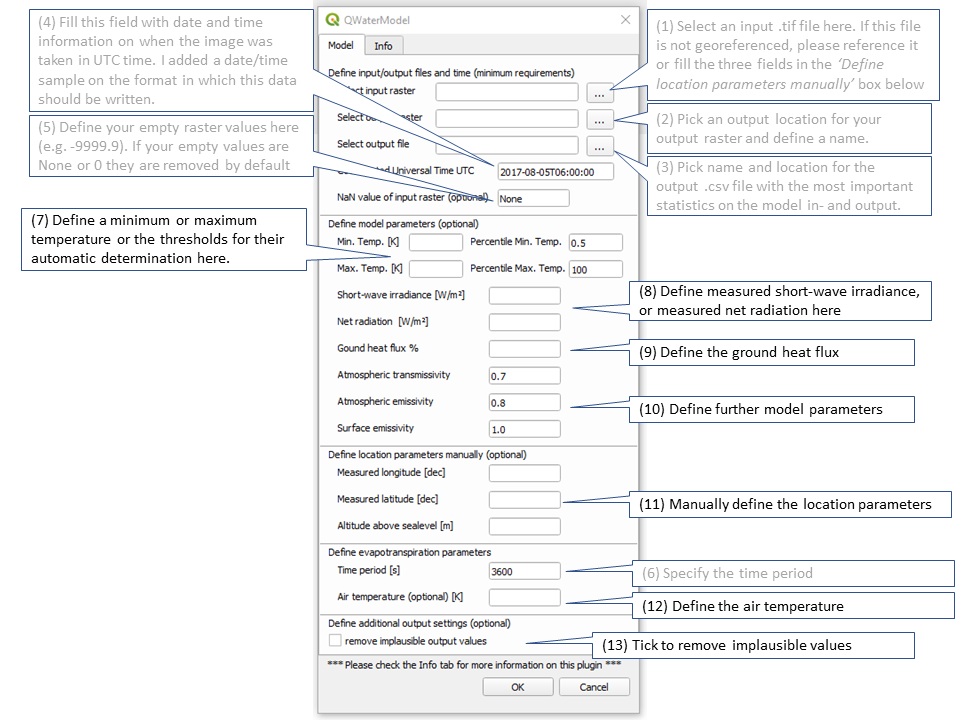
(8) As mentioned already above, clouds play a major role in the accurate determination of evapotranspiration when using thermal images. It is therefore very useful to measure incoming short-wave solar radiation too. Ideally both incoming and outgoing short- and long-wave radiation are measured, resulting in a radiation budget, the net radiation. If you have any of these measurements available, it is very recommendable to provide them here as input too.

(9) The ground heat flux is the amount of energy that is transferred from the surface to the soil. In dense forests, this flux is usually very low, because most of the energy remains in the tree canopy or is absorbed from the dense vegetation below. If there is very little vegetation and a large area of soil is exposed, more energy is transferred to the soil. Here you can input your measurements or estimates of the soil heat flux in %. If this box remains empty, the ground heat flux is estimated automatically.

(10) There are a few other parameters that can be specified. The defaults for atmospheric transmissivity and atmospheric emissivity usually work quite well. However, the value for surface emissivity is a rough simplification. Highly vegetated landscapes usually have a surface emissivity of 0.98, bare soil is usually lower.

(11) Usually your thermal image or map already comes with a geolocation. However, if this is not the case, e.g. because you are taking pictures with a handheld thermal camera, you can specify the longitude and latitude and the altitude above sea level here. Please make sure that you specify the coordinates in decimal degrees (e.g. the coordinates for Jakarta would be longitude: 106.7676 and latitude: -6.1911) and the altitude in meters.

(12) Finally, you can add a measured air temperature value. If this box is empty, the air temperature is simply estimated.

(13) A rather still experimental add-on is the removal of implausible output values. This removes values that are physically not possible.

Click the “OK” button to run QWaterModel. Your raster is saved as a .tif file and the statistics are saved in a .csv file in the location that you specified in step (2 and 3).

Did you encounter problems? Or did you find a bug?

I am always happy to help and I am even happier to remove bugs from the software. Just write me an email via the contact form.

How to cite QWaterModel

Ellsäßer et al. (2020), Introducing QWaterModel, a QGIS plugin for predicting evapotranspiration from land surface temperatures, Environmental Modelling & Software, https://doi.org/10.1016/j.envsoft.2020.104739.

Please also cite the DATTUTDUT energy-balance model on which this plugin is based:

Timmermans, W.J., Kustas, W.P., Andreu, A., 2015. Utility of an automated thermal-based approach for monitoring evapotranspiration. Acta Geophys. 63, 1571–1608. https://doi.org/10.1515/acgeo-2015-0016.

More Information

QWaterModel is the result of some rainy evenings during my PhD studies in 2019 and 2020. I realized that there was no simple tool for evapotranspiration estimation and modelling out there, that was simple to use, easy to access and open source. I don’t claim that it is perfect yet and due to its simplicity, I cannot guarantee that it will work under all conditions. If you have any suggestions, ideas for improvement or further development, did you find a bug or do you want to contribute to the QWaterModel project, please feel free to contact me via the contact form.

You can find the QWaterModel repository here.